Core Methods and Data Objects

Eurostat’s Deliverable D2.3 Volume III documents the algorithms, quality checks, and data contracts that make up the MultiMNO reference pipeline. The volume specifies, in detail, the full set of methods and data objects developed for four core use cases: Present Population Estimation, M-Usual Environment Indicators, M-Home Location Indicators, and Internal Migration. These methods sit underneath the framework (Vol. I) and use case catalogue (Vol. II) already summarised in this section of the docs. Telcofy keeps the same modular structure so that regulators can trace every output back to an ESS-aligned procedure. (Additional background is available via the CROS deliverables overview.)

• M-Home Location Indicators: derived from long-term permanence outputs, this pipeline labels each device’s de facto residence, aggregates counts to grids or administrative areas, and attaches quality/confidence scores plus change flags so downstream processes (e.g., internal migration) can quantify relocations.

1. Network topology & coverage modules

Module 1 — MNO network topology data cleaning (syntactic checks)

The first module scrubs raw topology feeds (cell plan CSV, JSON, XML) into the canonical schema. Validation falls into three buckets:

• Coordinate hygiene — latitude/longitude must exist, be parseable as WGS 84, and fall inside the bounding geometry provided for the target country. Optional altitude and antenna height are checked against admissible ranges (e.g. metres above sea level).
• Antenna descriptors — directionality, azimuth, elevation, power, beam widths, frequency, technology, and cell type are individually verified for presence (if required), data type, and inclusion in the enumerated value sets delivered with D2.3.
• Geometry payloads — when MNOs supply polygons (Cell Footprint with Differentiated Signal Strength Coverage Areas), Well Known Text is parsed and clipped to the bounding box; signal strength attributes must lie in the interval (0, 1].

Rows failing mandatory-field checks are dropped; optional-field failures are nulled but logged. The method emits:

• Clean MNO Network Topology Data — the sanitised dataset with type-correct columns ready for downstream geospatial joins.
• MNO Network Topology Data Quality Metrics — counts of rows removed per validation rule plus the k most frequent error signatures, so recurring issues can be negotiated with the operator.

Module 2 — MNO network topology quality warnings

Module 2 turns the metrics above into actionable warnings. For each topology refresh (typically daily), key series such as raw row count, post-clean row count, and field-level error ratios are tracked and compared with historical behaviour over a configurable look-back window (week, month, or quarter). Threshold types include:

• Absolute — e.g. “raise a warning if the number of cells falls below 10 000”.
• Relative — e.g. “raise a warning if today’s error rate exceeds the trailing mean by 30 %”.
• Control limits — control-chart style bands computed as μ ± k·σ.

Warnings are grouped by metric (size, missing values, wrong format, out-of-range, parsing errors) and the output dashboard plots the time series with annotated breaches so analysts can distinguish genuine network changes from ingest glitches. All thresholds can be tuned per NSI; defaults follow the values published in D2.3.

Module 3 — Signal strength estimation

When only the radio plan is available, Module 3 synthesises a radio-frequency coverage surface. Two variants are documented in D2.3; Telcofy implements both.

3.1 Omnidirectional model

For small cells or sectors with no directional beam, the received signal strength for cell a at grid tile g is

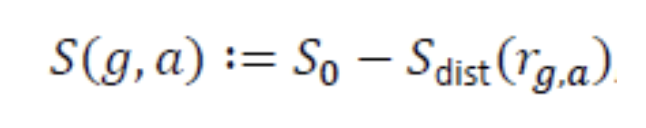
where:

• S₀ is the transmit power expressed as signal strength at reference distance r₀ = 1 m (converted from the cell plan power P in Watts via the standard Watt ↔ dBm conversion).
• r_{g,a} is the 3‑D distance between the antenna position and the tile centroid (assuming user devices at ground level).
• S_{\text{dist}}(r) encodes the distance-based attenuation:

with path-loss exponent γ describing reflections, diffraction, and clutter (default γ = 2 for free space, configurable for urban/rural scenes).

3.2 Directional model

Macrocells add angular attenuation. Let φ_a be the azimuth, θ_a the downtilt, α_a the horizontal 3 dB beam width, and β_a the vertical 3 dB width. Define:

• δ_{g,a} — difference between φ_a and the azimuth from cell a to tile g.
• ε_{g,a} — elevation offset between θ_a and the line of sight to tile g.

The directional signal model becomes

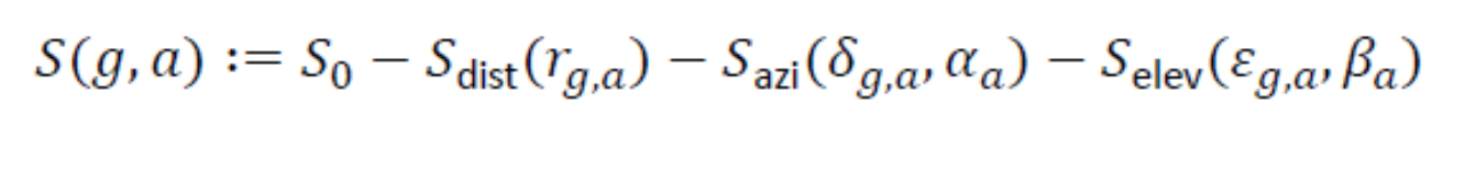
where S_{\text{azi}} and S_{\text{elev}} are Gaussian-shaped attenuation functions calibrated so that the loss reaches 3 dB at φ_a ± α_a/2 and θ_a ± β_a/2, respectively. D2.3 derives these functions by solving for the parameters c and σ in

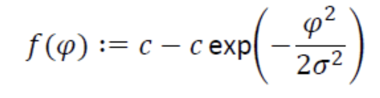
subject to the 3 dB constraints for each plane.

Figure 2 summarises the resulting radiation pattern: the main lobe is centred on the beam direction, grey rings indicate successive 5 dB loss levels, and the red arms mark the 3 dB beam limits (spanning 2α_a horizontally and 2β_a vertically). Side or back lobes may arise in real hardware, but the Gaussian attenuation captures the dominant behaviour used for downstream modelling.

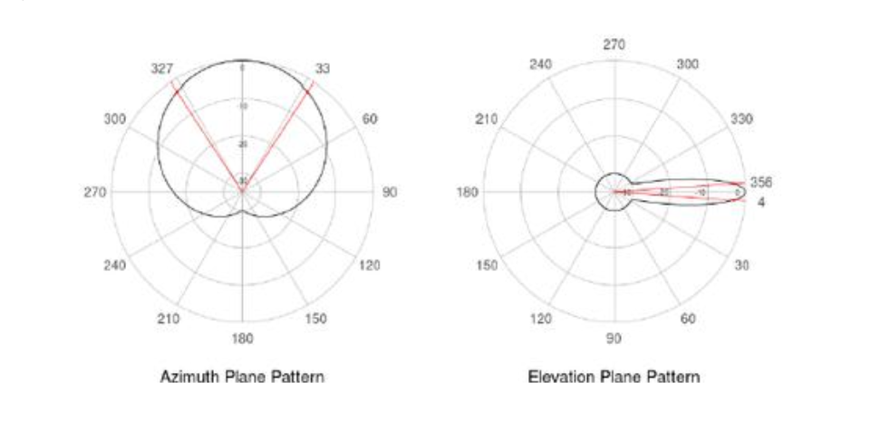Source: MultiMNO D2.3 Vol. III, Figure 2.

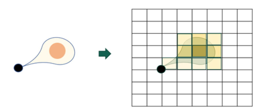
Once S_{g,a} is known, the coverage surface is rasterised onto the project grid by intersecting the continuous footprint with target tiles—see Figures 3–5 for the projection workflow extracted from D2.3. Figure 4, in particular, shows how arbitrary coverage shapes are snapped to the project_grid_cell lattice by attributing a specific strength (or other cell property) to every intersected tile.

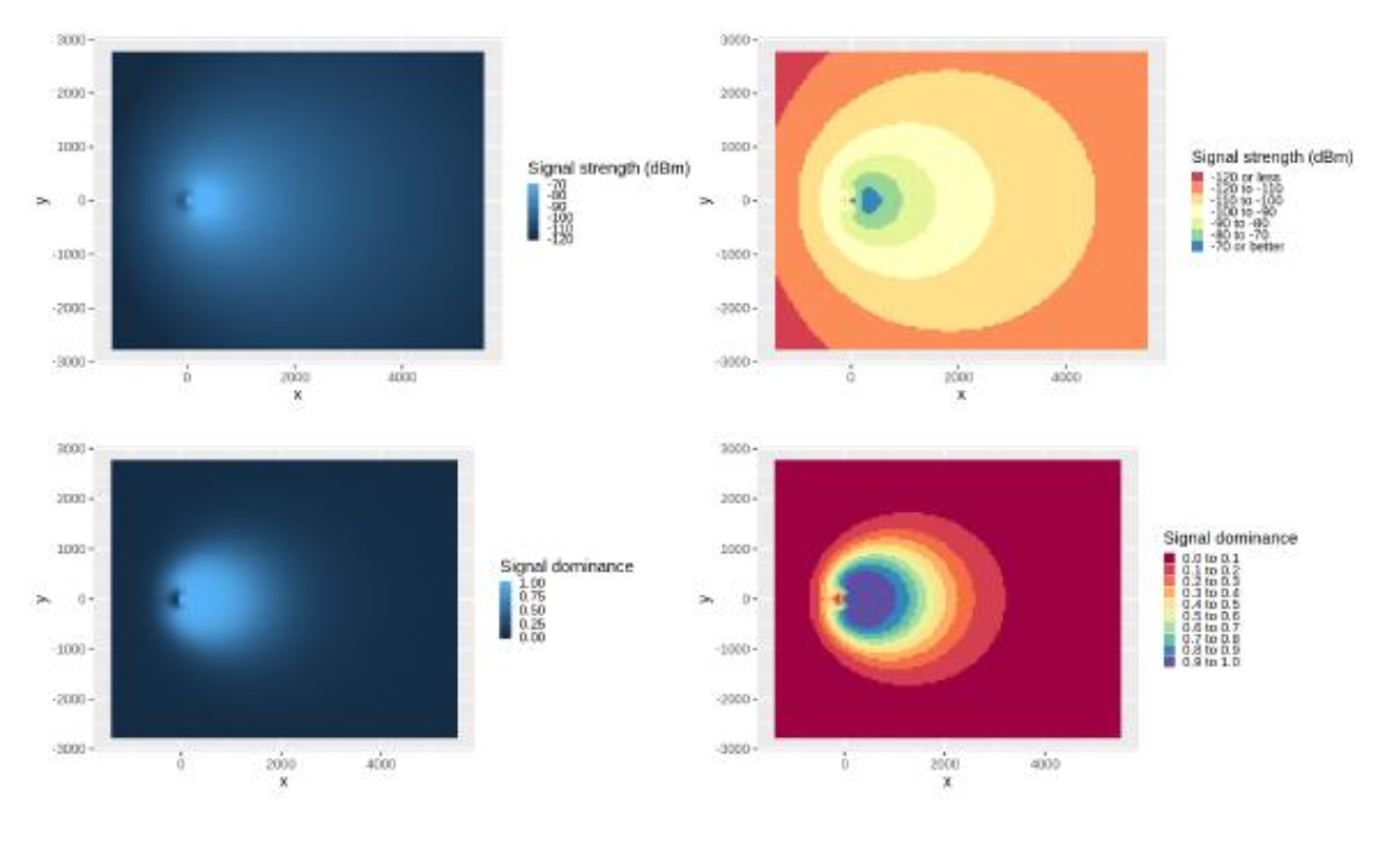Source: MultiMNO D2.3 Vol. III, Figure 3. Here the cell (located at x = 0, y = 0, height = 55 m, γ = 4, power = 10 W, azimuth pointing east, tilt = 5°, horizontal width = 65°, vertical width = 9°) produces peak signal a few hundred metres from the mast because tiles directly underneath have larger elevation offsets ε_{g,a}.

Source: MultiMNO D2.3 Vol. III, Figure 4.

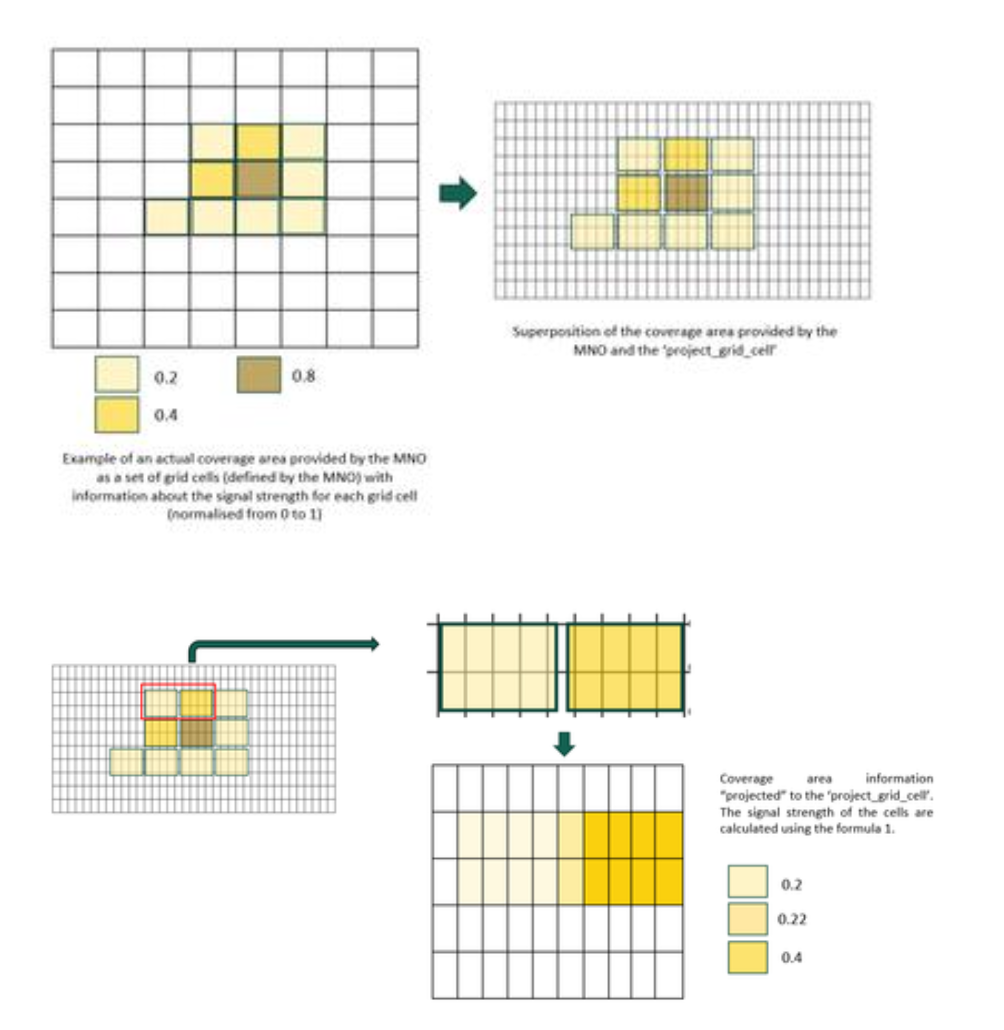Source: MultiMNO D2.3 Vol. III, Figure 5. The graphic demonstrates Equation 1 (below): intersect each MNO tile with the project_grid_cell, compute the overlap area A_{ij}, and aggregate the MNO strengths SE_j into the project tile i.

3.3 Precomputed signal-strength tiles

When the operator already supplies gridded signal strengths, Module 3 reprojects them. For each project tile i, intersecting with n MNO tiles, the blended signal is obtained using Equation 1 (below).

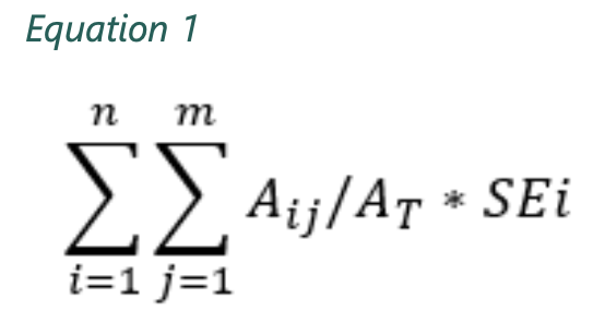
Here A_{ij} is the overlap area between project tile i and MNO tile j, A_T is the area of tile i, and S_j is the strength attached to MNO tile j.

Module 4 — Cell footprint estimation

Signal strengths are converted to dimensionless footprint values s(g,a) in the range [0,1], representing a cell’s relative suitability at tile g. D2.3 offers two transformation families:

• Linear

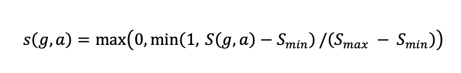
with default S_{\min} = -130 \text{dBm} and S_{\max} = -50 \text{dBm}.

• Logistic

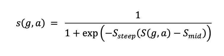
mirroring the “signal dominance” concept in Tennekes & Gootzen (2022). Parameters S_{\text{steep}} and S_{\text{mid}} control the knee of the curve; defaults (-92.5,\;0.2) capture typical macro-cell behaviour.

To keep the dataset tractable, the module prunes low-utility cells per tile. A simple threshold (e.g. s < 0.01) is available, but D2.3 recommends keeping only the Top‑X cells (default X = 10) for each tile:

Module 5 — Cell connection probability estimation

Footprint values become probabilistic connection weights assuming no load balancing:

where A is the set of all cells that reach tile g. For every tile the probabilities sum to one and serve as priors for later Bayesian localisation (Module 6). The outputs are stored as Cell Connection Probabilities [INTERMEDIATE RESULTS].

Reference: Tennekes, M. & Gootzen, Y. (2022). Bayesian location estimation of mobile devices using a signal strength model. Journal of Spatial Information Science.

2. Event-level quality assurance

• Module 7 – Event data syntactic cleaning
  Deduplicates records, orders events temporally, validates mandatory fields, and harmonises roaming identifiers.
• Module 8 – Event syntactic quality warnings
  Computes error rates and completeness metrics; emits daily dashboards with configurable thresholds.
• Module 9 – Device demultiplex
  Splits cleaned events into per-device streams, aligning by user ID and timestamp while preserving metadata needed downstream.
• Module 10 – Device-level semantic cleaning
  Removes impossible jumps (speed constraints, missing cells), imputes short gaps, and tags residual anomalies.
• Module 11 – Device activity statistics
  Derives per-device indicators (event counts, idle gaps, night/day ratios) used for filtering and weighting.
• Module 12 – Device semantic quality warnings
  Aggregates Module 10 & 11 scores into warning flags that can pause a pipeline or trigger manual review.

3. Daily & longitudinal analytics

• Module 13 – Daily processing
  Offers three interchangeable methods: present population estimation, daily permanence score, and continuous time segmentation (CTS). Each consumes semantically cleaned events and connection probabilities to produce daily summaries and state labels.
• Module 14 – Mid-term processing
  Aggregates daily permanence scores into monthly or quarterly summaries; implements decay rules, holiday adjustments, and confidence scores.
• Module 15 – Long-term processing
  Builds yearly permanence and usual-environment labels, including home/work classification, stay frequencies, and uncertainty indicators.
• Module 16 – Tourism methods
  Adapts daily outputs for inbound/outbound tourism: trip detection, nights spent, multi-destination chains, and country-of-origin logic. Validates robustness against multi-roaming scenarios.

4. Aggregation, fusion & estimation

• Module 17 – Device filtering & single-MNO aggregation
  Applies quality filters (minimum activity, residence confirmation) and aggregates devices to grid/time buckets with disclosure-aware measures.
• Module 18 – Merge single-MNO aggregates
  Combines results from participating MNOs using either secure enclave fusion or exchange of already-protected aggregates; harmonises schemas and metadata.
• Module 19 – Projection to use-case geography
  Projects grid counts to administrative or analytical zones (LAU, municipality, FUA) using the same spatial transformation rules referenced in Vol. I.
• Module 19 (Estimation stage) – Calibration of outputs
  Scales MultiMNO totals to official population frames via reweighting, residual adjustments, and estimation of coverage gaps (includes default inference recipes per use case).
• Home-location change detection (Chapter 22)
  Detects migrations by comparing sequential long-term labels with stability thresholds, enabling internal migration statistics.

5. Data objects catalogue

Volume III concludes with a detailed schema inventory (Chapter 23) covering:

• Input data – raw network topology, event logs, auxiliary datasets (holidays, MCC/MNC mappings, land use priors).
• Intermediate results – every bronze/silver artefact referenced in the pipeline (cleaned events, quality metrics, grid probabilities, daily/mid-term/long-term summaries).
• Output datasets – gold tables per use case, each with mandatory metadata (time period, spatial reference, quality flags, disclosure level).

Telcofy implementation notes

1. Module parity — keep the same numbering in code repositories and documentation so auditors can cross-check against D2.3 Vol. III.
2. Configurability — surface key parameters (speed thresholds, permanence windows, calibration weights) in configuration files, mirroring Eurostat defaults but explicitly tracking Telcofy overrides.
3. Quality evidence — persist syntactic and semantic warning outputs; these artefacts demonstrate compliance with the ESS quality framework and feed customer-facing dashboards.
4. Privacy controls — respect the separation between single-MNO processing, secure enclaves, and post-aggregation SDC as defined in Modules 17–20. Telcofy add-ons must not bypass these boundaries.

See D2.3 Vol. III for algorithmic detail, pseudocode, and full attribute definitions.